| Issue |
Natl Sci Open
Volume 4, Number 3, 2025
|
|
|---|---|---|
| Article Number | 20240045 | |
| Number of page(s) | 20 | |
| Section | Engineering | |
| DOI | https://doi.org/10.1360/nso/20240045 | |
| Published online | 13 January 2025 | |
RESEARCH ARTICLE
Two-group bubble size distribution evolution in vertical two-phase flow: Mechanistic model development and evaluation in a tight-lattice rod bundle
1
School of Mechanical Engineering, Shanghai Jiao Tong University, Shanghai 200240, China
2
Key Laboratory of Nuclear Power Systems and Equipment of the Ministry of Education, Shanghai Jiao Tong University, Shanghai 200240, China
3
Department of Mechanical Engineering, City University of Hong Kong, Hong Kong 999077, China
4
State Key Laboratory of Nuclear Power Safety Technology and Equipment, Shanghai Jiao Tong University, Shanghai 200240, China
* Corresponding authors (emails: This email address is being protected from spambots. You need JavaScript enabled to view it.
(Yao Xiao); This email address is being protected from spambots. You need JavaScript enabled to view it.
(Hanyang Gu))
Received:
24
August
2024
Revised:
10
December
2024
Accepted:
9
January
2025
Abstract
Two-phase flow with complex phase interfaces is commonly observed in both nature and industrial processes. The bubble size distribution (BSD) is a crucial parameter in gas-liquid two-phase flow, impacting various flow characteristics including interfacial forces, void fraction distribution, and interfacial area transport. Throughout the flow progression, the BSD changes along the channel due to variations in pressure and interactions among bubbles. Accurately predicting the evolution of BSD can enhance the modeling of two-phase flow. This study presents a novel BSD evolution (BSDE) model, where the governing equation for the probability density function is formulated by considering the conservation of bubbles within a one-dimensional control volume in the channel. The downstream BSD is predicted based on the upstream BSD and the effects of pressure variations and bubble interactions along the channel. To account for the multiscale nature of the two-phase flow, the bubbles are categorized into small groups (G1) and large groups (G2). Six distinct source term distributions for intra/inter bubble interactions have been developed. Each source term accounts for the distributions of consumed and generated bubbles, ensuring the conservation of bubble volume through constraints on model coefficients. The model has been tested on a tight-lattice rod bundle using experimental data, with deviations of less than 5% and 15% for G1 and G2 flow, respectively. Since the model development is independent of specific geometry, the framework of the BSDE model can also be effectively applied to channels of varying shapes.
Key words: bubble size distribution evolution / bubble interactions / two-phase flow / interfacial area concentration / tight lattice rod bundle
© The Author(s) 2025. Published by Science Press and EDP Sciences.
 This is an Open Access article distributed under the terms of the Creative Commons Attribution License (https://creativecommons.org/licenses/by/4.0), which permits unrestricted use, distribution, and reproduction in any medium, provided the original work is properly cited.
INTRODUCTION
The occurrence, development, and dissipation of bubbles within two-phase flow phenomena are prevalent in both natural environments and a variety of industrial applications, as illustrated in Figure 1. Examples include the processes of water boiling and condensation, chemical engineering practices, and nuclear systems [1–3]. Bubbles serve as versatile carriers with significant potential for applications such as enhancing boiling heat transfer [4], targeted cancer treatment [5], and controlling nanofluidic transport [6]. Furthermore, in fluid physics, the microscopic dynamics of multiscale bubbles play a crucial role in shaping the macroscopic characteristics of two-phase flow, such as interphase energy-mass transfer area [7], two-phase distributions in the flow field [8], bubble interactions, and transitions of flow patterns [9]. Consequently, the distribution of bubble sizes is of paramount importance. Previous studies have shown that bubbles of varying sizes exhibit distinct dynamic characteristics [7,8,10–13]. As an illustration, consider the two-phase flow in a small pipe with an inner diameter of 30 mm at room temperature (25°C) and normal pressure (0.1 MPa). Under low gas content, the gas phase is characterized by small, spherical bubbles that may exhibit distortion. As pressure decreases and gas content increases, the coalescence and expansion of these small bubbles facilitate the emergence of cap-shaped and slug bubbles throughout the channel’s cross-section. Furthermore, the lift force [8] influences the migration of small discrete bubbles toward the low-velocity region and the movement of large cap-shaped and slug bubbles toward the high-velocity region in a continuous phase flow field. The distribution characteristics of bubbles of varying sizes at the micro-scale indicate the macroscopic phase distribution characteristics under different flow patterns. Meanwhile, bubbles of different sizes exhibit varying rising velocities. Combining these factors, the interactions between multi-scale bubbles and their impact on the surrounding flow field vary, with large bubbles typically creating low-pressure wake regions behind them [14]. In these wake regions, smaller bubbles may accelerate and merge with larger bubbles, leading to a dynamic interfacial structure that contributes significantly to the complexity of two-phase flow evolution.
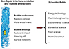 |
Figure 1 Bubble dynamic behavior with flow evolution and its potential occurrence scenarios. |
Notably, in industrial systems involving two-phase flow, the mass, momentum, and energy transfer of the two phases occur through the phase-interface structure [15]. Accurate characterization of the phase-interface structure in such systems is crucial for optimizing system design and enhancing system security. As discussed previously, the bubble size essentially influences the magnitude of the phase-interface structure [14]. For instance, in a two-phase flow system with consistent gas phase content, the small bubbles’ presence results in a larger phase interface area within the unit spatial control volume (Interfacial Area Concentration, IAC). Conversely, larger bubbles lead to a smaller phase interface area. To predict the evolution of the phase interface, researchers developed the interfacial area transport equation (IATE) [16]. IATE takes IAC as the transport object, dynamically predicting the IAC evolution by considering the bubbles’ coalescence, break-up, evaporation, condensation, etc. [17]. Initially, Wu et al. proposed an IATE model for the bubbly flow. Subsequently, Fu [18] and Sun [19] extended the IATE model further to the slug flow and churn-turbulent flow by dividing the bubbles into two groups to establish bubble-interaction models (the group-1 bubbles G1, referring to small and distorted bubbles; the group-2 bubbles G2, referring to cap and slug bubbles). Up to now, IATE has been further extended from the simple pipe and rectangular to the complex rod bundle channel [20]. Recently, a growing concern has been that the current IATE model is unable to give satisfactory predictions in the transition from the bubbly flow to the slug flow [17]. To overcome such a flaw of the current IATE, researchers have developed wake entrainment models combined with a hypothetical bubble size distribution (BSD) [21,22]. Essentially, the IATE model flaw described above is because the model was developed based on the flat number density distribution of bubbles [14]. In the flow-pattern transition, BSD varies dramatically, which leads to drastic changes in the IAC and void fraction. Consequently, precise micro-scale bubble size distribution evolution (BSDE) prediction is crucial for accurately characterizing the IAC and void fraction evolution, which is also meaningful in describing other two-phase flow behaviors in both natural and industrial settings.
This study introduces a mathematical model, known as the BSDE model, which accounts for the transportation of bubble particles. The bubbles are categorized into two groups like that in the two-group IATE, to address the multiscale nature of bubbles in the BSDE model. The model development incorporates considerations of pressure variation, as well as bubble coalescence and break-up to capture their effects on the BSDE. To characterize bubble interactions, the bubble coalescence due to random collision (RC) and wake entrainment and the bubble break-up due to turbulent vortex and flow-field shearing-off are considered in the BSDE model. The model’s performance is assessed using BSD data obtained within a tight lattice bundle channel under gas-liquid flow conditions. The results show that the BSDE model can accurately predict the evolution of bubble sizes, with a deviation of 5% for one-group flow and 15% for two-group flow.
FRAMEWORK OF THE GENERAL BSDE MODEL
General remarks
For the two-phase flow in a general channel geometry, the bubble interactions affect the evolution of the bubble size. In addition, when considering the gravity head and friction resistance, the pressure gradually decreases along the axial direction, resulting in an increase in the bubble size along the channel. According to the upstream BSD, the downstream BSD can be predicted by considering the bubble coalescence/break-up and the pressure variation along the channel, which is the principle of the BSDE model. Given significant differences in the hydraulic behavior and interactions between the small and large bubbles, the bubbles were divided into two groups according to the critical size, as denoted by Equation (1), to consider the bubble interaction between the different scales. The feasibility of the two-group bubble division has been widely verified in the two-group IATE model [21–23]. As a theoretical derivation, the framework of the general BSDE model in this section is derived based on a vertical gas-liquid two-phase flow in a small- or medium-sized pipe under a 1-D steady state. However, it should be noted that the proposed BSDE model can be applied to other geometric flow channels theoretically whose hydraulic diameter is equivalent to that of small- or medium-sized pipe, after combining the geometry characteristics of the specific flow channel.
 (1)
(1)
Governing equation of the PDF for BSD
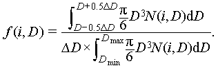
As mentioned above, the current BSDE model was developed by considering the effect of pressure and bubble coalescence/break-up during the flow evolution. The schematic of the 1-D control volume of a vertical channel is shown in Figure 2. The upstream face of the control volume is marked as the i-th face, and the downstream face is marked as the i+1-th face. The cross-sectional area of the channel is represented as A (m2); the axial length of the control volume is Δz (m); the void fraction at the i-th face is α(i); the velocity of the bubbles with diameter D at the i-th face is vg(i, D) (m/s); the proportion of bubbles within diameter (D − 0.5ΔD, D + 0.5ΔD) at the i-th face is f(i, D) × ΔD. The symbol ΔD represents the differential of D. f(i, D) is the PDF of BSD at the i-th face, indicating that, in the unit space, the proportion of bubbles located in different diameter intervals in the volume of the total bubbles:
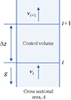 |
Figure 2 One-dimensional control volume. |
 (2)
(2)
During time Δt, the total volume of bubbles within (D − 0.5ΔD, D + 0.5ΔD) passing through the i-th face is marked as Gi:
 (3)
(3)
Further, during Δt, the total volume of bubbles within (D − 0.5ΔD, D + 0.5ΔD) passing through the i+1th face is marked as Gi+1 (m3):
 (4)
(4)
With pressure variation, the bubbles will expand or contract. From the i-th face to the i+1-th face, the increase in the total volume of bubbles within (D − 0.5ΔD, D + 0.5ΔD) due to the pressure effect is denoted as Gp (m3):
 (5)
(5)
where Pi and Pi+1 are the absolute pressures at the i-th and i+1-th faces, respectively. vg is an independent parameter, similar to IATE model [24], which can be obtained by experiment or from the momentum if the current model is combined with the two-fluid model. In addition, the introduction of the velocity indicates that Equation (5) also contains the velocity effect on BSD evolution.
With bubble coalescence and break-up, the increase in the total volume of bubbles within (D − 0.5ΔD, D + 0.5ΔD) is denoted as GS (m3):
 (6)
(6)
where  is the BSD source term for the j-th bubble interaction mechanism at the i-th face (1/(m s)).
The conservation equation of bubble volume concerning bubble size of (D − 0.5ΔD, D + 0.5ΔD) in the control volume can be written as
 (7)
(7)
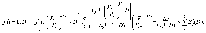
Rearrange Equation (7) as
 (8)
(8)
In Equation (8), the LHS (Left-hand Side) is the BSD at the downstream node, and the RHS (Right-hand Side) represents the function of the upstream BSD. The first term on the RHS is the BSD source for the variation in pressure and bubble velocity, and the second term denotes the BSD source for the bubble coalescence and break-up. Equation (8) clearly shows the principle of the BSDE model, based on the BSD information at the upstream node, considering the effects of bubble velocity change, pressure change, and bubble interactions on BSD, to predict the BSD downstream.
Source terms for bubble interactions
For a realistic two-phase flow, the mechanisms of bubble coalescence and breakup can be divided into five categories, which affect the BSD evolutions, as shown in Figure 3: (a) bubble coalescence due to RC driven by turbulent vortices; (b) absorption of the trailing bubble by the leading bubble owing to wake entrainment (WE); (c) bubble breakup due to turbulent impact (TI); (d) shearing off (SO) of a large number of small bubbles from the tail of a large bubble; (e) large bubble breakup due to surface instability (SI). Given the different effects of channel size (hydraulic diameter) on multi-scale bubbles, the above bubble interaction mechanism does not usually occur simultaneously. For the two-phase flow in the small- and medium-sized pipes concerned in this study, unimportant bubble interaction mechanisms should be excluded during the development of the model. Specifically, in the small- and medium-sized channels, the G2 bubbles’ size is in the same order of magnitude as the channel cross-section. The random movement of G2 bubbles driven by the turbulent vortex is not significant. In addition, the RC sub-mechanisms that involved G2 bubbles can be ignored (RC(12, 2) and RC(2)). According to experimental observations, in the medium-size channel, the probability of G2 bubbles breaking up owing to TI and SI is small; in addition, the breakup mechanisms of G2 bubbles can be ignored (TI(2, 11), TI(2, 12), TI(2), SI(2)). The remaining mechanisms were simulated: RC(1), RC(11, 2), WE(1), WE(11, 2), WE(12, 2), WE(2), TI(1), and SO(2, 12) (Supplementary information). However, given the complexity of the real two-phase flow, the neglected source/sink terms may also have important effects on the BSD evolution under different flow conditions and channel geometry. In addition, the current development of the source/sink model assumes the range of bubble sizes applicable to different models, which is also a source of error. Nevertheless, the current data evaluation results prove the rationality and feasibility of the current modeling strategy. In future studies, more data from different flow conditions and channel geometries will be needed to verify and optimize the model’s performance.
 |
Figure 3 Mechanisms of bubble coalescence and breakup. (a) RC; (b) WE; (c) TI; (d) SO; (e) SI. |
Derivation method of undetermined coefficients and BSDE model assessment criteria
During the development of the BSDE model, undetermined coefficients were introduced in the submodel of each source term, including CRC1_1 in the G1 bubble coalescence due to RC, CWE1_1 in the G1 bubble coalescence due to wake entrainment, CWE2_1 in the G2 bubble coalescence due to wake entrainment, CWE21_1 in the G1 and G2 bubble coalescence due to wake entrainment, CSO21_1 in the G2 bubble SO, and CTI1_1 in the G1 bubble breakup due to TI. After the undetermined coefficients are determined based on the bubble interaction dominant experimental results, the BSDE model can be experimentally evaluated. The schematic of the computational scheme of the BSDE model is shown in Figure 4.
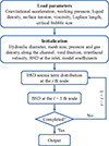 |
Figure 4 Schematic of the computational scheme of the BSDE model. |
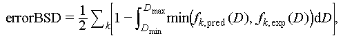
To quantify the differences between the experimental results and the theoretical predictions, the relative error was determined by the area surrounded by the experimentally measured BSD, the model-predicted BSD, and the x-axis, as shown in Figure 5. In Figure 5, a larger shadowed area would imply a more accurate model. The expression of the model relative error is
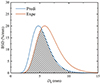 |
Figure 5 Relative error in BSD prediction. |
 (9)
(9)
where fk,pred(D) is the BSD from the model prediction at the k-th port, and fk,exp(D) is the experimentally obtained BSD at the k-th port.
APPLICATION OF THE BSDE MODEL TO A TIGHT-LATTICE ROD BUNDLE AND EVALUATION
In this section, the BSDE model proposed in Section “Framework of the general BSDE model” was applied to predict the BSD evolution in a specific tight-lattice bundle. The experimental database, model coefficients derivation, and prediction results were discussed in the following.
Experimental database and coefficients derivation
The experimental data were from a dual sub-channel tight lattice rod bundle, whose flow conditions are shown in Figure 6, including the bubbly flow, cap-bubbly flow, and slug flow. The experiments used a dual wire-mesh sensor to measure the phase interface information with a high resolution shown in Figure 7 and to acquire the void fraction, BSD, IAC, and bubble velocity with the Maxwell No Cut method [25] and self-developed Eulerian post-processing algorithm [26]. Figure 8 shows the typical BSD evolution experimental results. The pressure data at the measurement ports were also recorded through differential pressure transmitters. More details can be obtained from the previous research [13]. By linear interpolation, the flow parameters, including the group-wise bubble velocity, void fraction, and absolute pressure along the channel axial direction, were calculated based on the experimental data. This avoids the effects of model uncertainty in predicting these parameters on the BSDE model. The BSDs measured in the experiments at z/Dh = 57.90 were used as the inlet boundary of the BSDE model, and the experimental data at z/Dh = 86.86 and 115.8 were used for fitting the BSDE model coefficients and evaluating the model. The calculation method of BSD can be referred to from Refs. [26,27].
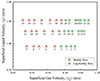 |
Figure 6 Experimental flow conditions at z/Dh = 115.8. |
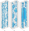 |
Figure 7 3-D phase interface distribution in the tight lattice bundle based on the WMS technique. (a) Bubbly flow; (b) cap-bubbly flow; (c) slug flow [28]. |
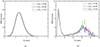 |
Figure 8 Typical BSD evolution experimental results. (a) One-group flow, case 20; (b) two-group flow, case 11. |
The model coefficient is determined according to the dominant flow condition of the mechanism. It is worth mentioning that the BSDE model requires the geometrical information of G2 bubbles to calculate the BSDE source term from the SO of a G2 bubble (SO(21)). Given the absence of modeling of bubble geometric characteristics in the current study, to ensure the integrity of the model, the fitting correlations obtained from the experimental data were used [29] to calculate the G-2 bubbles’ height and projected area diameter, as shown in Equations (10) and (11). This does not affect the overall model framework’s valuation and the source/sink terms’ functionality evaluation. These experimental data were also used for the BSDE-model evaluation in Sections “Evaluation in one-group flow conditions” and “Evaluation in two-group flow conditions”.
 (10)
(10)
 (11)
(11)
The following is the coefficient fitting process. It follows the IATE model coefficient confirmation strategy, where the experimental data for fitting the undetermined coefficients and evaluating the model were not distinguished [21,30,31]. First, the experimental data for one-group flow were used to fit the coefficients in the G1 bubble interaction mechanisms. Six flowing conditions of one-group flow, with different superficial liquid velocities, were selected to fit these coefficients. In cases 21, 32, and 35, the bubble size increases along the channel owing to bubble coalescence. These three conditions were selected to fit CRC1_1, with coefficients CTI1_1 and CWE1_1 set to zero. In cases 8, 16, and 30, the effects of bubble coalescence on global BSD were compensated by the bubble breakup due to TI. These three flowing conditions were used for CTI1_1, with CWE1_1 set to zero. Although the source term distribution of WE(1) was developed, WE(1) has a negligible influence on the experimental data of BSDE. Therefore, the effects of WE(1) were incorporated into RC(1), and the coefficient CWE1_1 was set to zero. After CTI1_1 was fitted, CRC1_1 was refitted with the updated CTI1_1 and into the next fitting loop until the values of CRC1_1 and CTI1_1 were stable.
Second, the coefficients of G2 bubble interactions were fitted after CRC1_1 and CTI1_1 were determined. Cases 1, 12, and 23 were selected to fit CWE2_1, with CSO21_1 and CWE21_1 set to zero. In these three conditions, the size of G2 bubbles was significantly larger owing to WE(2). In cases 11 and 24, a large number of G1 bubbles were generated by SO(21); therefore, these two flowing conditions are suitable for CSO21_1 fitting. Coefficient CWE21_1 was set to zero during CSO21_1 fitting. In cases 1 and 12, the generation of G1 bubbles from SO(21) was compensated by the consumption of G1 bubbles from WE(21). These two flowing conditions were used for CWE21_1 fitting. After CWE21_1 was fitted, CWE2_1 was refitted with the updated CSO21_1 and CWE21_1 and into the next fitting loop until the values of these three coefficients were stable.
The fitted coefficients are shown in Table 1.
Coefficients in the BSDE model
Evaluation in one-group flow conditions
The relative error of the BSDE model for one-group flow (bubbly flow) is shown in Figure 9. All the flowing conditions display a relative error smaller than 5%, indicating that the BSDE model has high accuracy for BSD prediction in the one-group flow. It is worth noting that the evolution of BSD in the upstream and downstream is insignificant, which is another reason for such a small deviation. The detailed BSD prediction results for cases 33, 18, and 6 are shown in Figures 10–12, respectively. Figures 10(a), 11(a), and 12(a) show the experimentally measured BSDs at different axial positions of the flow channel. Figure 10(b) and (c), Figure 11(b) and (c), and Figure 12(b) and (c) show the BSD comparison between the predicted and experimental measurements. Moreover, Figures 10(d), 11(d), and 12(d) show the BSD accumulation change caused by each source/sink term under different bubble diameters during the whole flow development process.
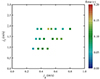 |
Figure 9 Model evaluation of one-group flow. |
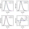 |
Figure 10 BSDE model evaluation under case 33, with jf = 1.86 m/s, jg = 0.11 m/s. (a) Experimental BSD; (b) model prediction vs. experiments for z/Dh = 86.86; (c) model prediction vs. experiments for z/Dh = 115.8; (d) accumulation of each source term along the channel length. |
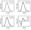 |
Figure 11 BSDE model evaluation under case 18, with jf = 1.39 m/s and jg = 0.16 m/s. (a) Experimental BSD; (b) model prediction vs. experiments for z/Dh = 86.86; (c) model prediction vs. experiments for z/Dh = 115.8; (d) accumulation of each source term along the channel length. |
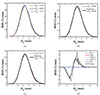 |
Figure 12 BSDE model evaluation under case 6, with jf = 0.93 m/s and jg = 0.17 m/s. (a) Experimental BSD; (b) model prediction vs. experiments for z/Dh = 86.86; (c) model prediction vs. experiments for z/Dh = 115.8; (d) accumulation of each source term along the channel length. |
For case 33, the peak value of the BSD at the first measured port (z/Dh = 57.90) appears at Db = 2.5 mm. With the flow development, the bubble size increases and the BSD profile shifts toward the right side. The peak value of the BSD at the third port (z/Dh = 115.8) appears at 2.8 mm, as shown in Figure 10(a). The comparison of the BSDs between the model prediction and experimental measurements for z/Dh = 86.86 and 115.8 are shown in Figure 10(b) and (c), respectively, displaying good consistency.
In the one-group flow, the bubble expansion and RC(1) are the dominant mechanisms for the BSD evolution. The bubble expansion shifts the BSD toward the right side, which in the source term distribution consumes small-sized bubbles and generates large-sized bubbles, which also implies the increment of the IAC. Figure 6(d) shows that bubbles with Db = ~2 mm were consumed and those with Db = ~4 mm were generated in RC(1). In addition, TI(1) consumed large bubbles and generated small bubbles. In case 33, with jf = 1.86 m/s, the fluctuation velocity is large enough for the breakup of bubbles with Db = 4–5 mm, as shown in Figure 10(d), and generates bubbles with Db = 3–4 mm. With the decrease in the superficial liquid velocity, the velocity of fluctuation decreases, the diameter of the broken bubbles increases, and the contribution of TI(1) decreases. For case 18, with jf = 1.39 m/s, only a few bubbles with diameters of approximately 5–6 mm are consumed due to TI(1) and that of generated bubbles is Db = 4–5 mm. For case 6, with jf = 0.93 m/s, the contribution of TI(1) can be ignored. As the BSD profile does not display perfect smoothness, the source term accumulation and distribution also show a certain degree of fluctuation.
Evaluation in two-group flow conditions
The relative error of the BSDE model for the prediction of a two-group flow is shown in Figure 13. All the flowing conditions show a relative error smaller than 15%, indicating that the BSDE model accurately predicts the BSDE along the channel. In a two-group flow, the effects of the G2 bubble coalescence due to WE(2) and SO on BSDE were significant. The BSDE was more significant for a two-group flow than for a one-group flow. The detailed BSD prediction results for cases 23, 10, and 1 are shown in Figures 14–16, respectively. Figures 14(a), 15(a), and 16(a) show the experimentally measured BSD at different axial positions of the flow channel. Figure 14(b) and (c), Figure 15(b) and (c), and Figure 16(b) and (c) show the BSD comparison between the model prediction and experimental measurements, respectively. Further, similar to that in the one-group flow conditions, Figure 14(d) and (e), Figure 15(d) and (e), and Figure 16(d) and (e) show separately the G1 and G2 BSD accumulation change caused by each source/sink term under different bubble diameters during the whole flow development process.
 |
Figure 13 Model evaluation of a two-group flow. |
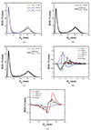 |
Figure 14 BSDE model evaluation under case 23, with jf = 1.86 m/s, jg = 0.70 m/s. (a) Experimental BSD; (b) model prediction vs. experiments for z/Dh = 86.86; (c) model prediction vs. experiments for z/Dh = 115.8; (d) accumulation of each source term on G1 bubbles along the channel length; (e) accumulation of each source term on G2 bubbles along the channel length. |
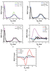 |
Figure 15 BSDE model evaluation under case 10, with jf = 1.39 m/s, jg = 0.68 m/s. (a) Experimental BSD; (b) model prediction vs. experiments for z/Dh = 86.86; (c) model prediction vs. experiments for z/Dh = 115.8; (d) accumulation of each source term on G1 bubbles along the channel length; (e) accumulation of each source term on G2 bubbles along the channel length. |
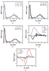 |
Figure 16 BSDE model evaluation under case 1, with jf = 0.93 m/s, jg = 0.49 m/s. (a) Experimental BSD; (b) model prediction vs. experiments for z/Dh = 86.86; (c) model prediction vs. experiments for z/Dh = 115.8; (d) accumulation of each source term on G1 bubbles along the channel length; (e) accumulation of each source term on G2 bubbles along the channel length. |
In a two-group flow, the bubbles were naturally divided into a small-size group and a large-size group, as shown in Figure 14(a). For example, consider case 23, in which the G1 bubbles show Db < 11 mm and the G2 bubbles show 20 < Db < 40 mm. The range of 11 < Db < 20 mm is the transition region with a few bubbles. With the flow development, the BSD profile of the G2 bubbles shifts toward the right side owing to WE(2), and the BSD profile of the G1 bubbles increases owing to SO(21). Therefore, the G2 IAC will decrease, and the G1 IAC will increase. In addition, the profile of G1 bubble BSD remains similar at different axial positions, proving the rationality of the assumption of the generated BSD concerning SO(21), as discussed in Supplementary Section 2.5. It was assumed that the BSD of the generated G1 bubbles from SO is proportional to the BSD of the G1 bubble at the current node.
The comparisons of BSD between the model prediction and experimental measurements for z/Dh = 86.86 and 115.8 are shown in Figure 14(b) and (c), respectively, displaying good consistency. The BSD variation characteristics of the bubbles in the two groups are reproduced by the BSDE model. The accumulation of each source term on the G1 bubbles is shown in Figure 14(d). Multiple bubble interaction mechanisms were activated and the SO(21), TI1, Expa, and RC1 are observed as the dominant mechanism for the G1-bubble BSDE. SO(21) is an intergroup mechanism, which consumed G2 bubbles and generated G1 bubbles. Although SO(21) is a dominant source term for the G1 bubble, it has a negligible effect on the G2 bubbles, as shown in Figure 14(e). For the G2 bubbles, the WE(2) and Expa is the dominant mechanism, which is consistent with the experimental observations. In WE(2), bubbles with 25 mm < Db < 35 mm were consumed, and bubbles with 35 mm < Db < 45 mm were generated.
In case 10, with jf = 1.39 m/s and jg = 0.68 m/s, a significant peak was observed in the BSD of the G2 bubble for z/Dh = 57.90 (as shown by the green line in Figure 15(a)). Most of the G2 bubbles had diameters ranging from 28 to 38 mm. These were observed under the flowing conditions near the flow regime transition boundary. Many G1 bubbles were generated at the inlet, and then drastic bubble coalescence occurred, resulting in small G2 bubbles with similar sizes. With the flow development, G2 bubbles coalesce owing to WE(2), and the BSD of the G2 bubble flattens further. The BSDE of the G2 bubbles was accurately predicted by the BSDE model, as shown in Figure 15(b) and (c). WE(2) was also the dominant mechanism for the G2-bubble BSDE, as shown in Figure 15(e). Bubbles with a diameter of 30–35 mm were consumed and bubbles with a diameter of 35–50 mm were generated. For the G1-bubble BSDE, the SO(21) was the dominant mechanism. The comparison results for case 1 are similar to those of cases 23 and 10, as shown in Figure 16. Thus, the BSDE characteristics were accurately predicted by the BSDE model. The SO(21) was the dominant mechanism for the G1-bubble BSDE and WE(2) was the dominant mechanism for the G2 bubbles. With the decrease in superficial liquid velocity, the fluctuation amount of the liquid velocity decreases, and the effects of TI(1) on the BSDE decrease. Therefore, the contribution of TI(1) was significant in case 23 with jf = 1.86 m/s, whereas it was weak in case 1 with jf = 0.93 m/s.
CONCLUSION
The BSD is a critical parameter in gas-liquid two-phase flow, significantly influencing characteristics such as void fraction and interfacial area. Pressure fluctuations and bubble interactions during flow progression result in BSDE along the channel. This study introduces a 1-D BSDE model to simulate the evolution of BSD along a vertical channel.
Due to the complex multiscale nature of the two-phase flow, bubbles are categorized into two groups to model the distribution of the bubble interaction terms. Six distinct bubble interaction mechanisms were developed in this study: (1) coalescence of G1 bubbles due to RC; (2) coalescence of G1 bubbles due to wake entrainment; (3) coalescence of G2 bubbles due to wake entrainment; (4) coalescence of G2 and G1 bubbles due to wake entrainment; (5) SO of G2 bubbles; and (6) G1 bubble breakup due to TI. Each mechanism encompasses the distributions of bubble consumption and production. Through coefficient constraints, it was determined that the total volume of consumed bubbles equaled the total volume of generated bubbles, ensuring conservation of bubble volume.
Experimental data from an air-water two-phase flow in a double sub-channel tight lattice rod bundle were utilized to calibrate the BSDE model and assess its precision. The flow region includes one-group bubbly flow and two-group cap-bubbly flow. The model inlet boundary was set at z/Dh = 57.90, with validation data obtained at z/Dh = 86.86 and 115.8. In the case of one-group flow, the BSD exhibited a single-peak profile with bubble sizes smaller than 11 mm, and the BSDE model’s prediction deviation was within 5%. The dominant mechanisms influencing the BSD evolution were identified as bubble expansion and RC(1), leading to a shift of the BSD towards higher values. In the case of two-group flow, the BSDE model’s prediction deviation was within 15%. The effects of the G2 bubble coalescence due to WE(2) and the G2 bubble breakup due to SO on BSDE were significant. With the flow development, the BSD profile of the G2 bubbles shifts toward the right side owing to WE(2), and the BSD profile of G1 bubbles increases owing to SO(21). The accurate predictions of BSDE demonstrate the feasibility of the proposed BSDE model.
The verification of the model presented in this study is based on data from a tight lattice rod bundle. It is worth noting that, the source/sink models of the BSDE model were developed based on the small- and medium-sized pipes. It implies that the current model can theoretically be extended to geometric channels of different cross-section shapes, as long as their hydraulic diameters are in the small- and medium-sized pipe category, with minor adjustments, as only the G2 bubble-shape assumption and SO mechanism are related to channel shape. Future research should evaluate the BSDE model’s accuracy using experimental data in basic geometric channels like circular or rectangular ones. Additionally, the void fraction distribution prediction model and IATE model should be improved based on the BSDE model in future studies.
Funding
This work was supported by the National Natural Science Foundation of China (12322510 and 12275174), the Shanghai Rising-Star Program (22QA1404500), the Science and Technology Commission of Shanghai Municipality (24DZ3100300), and the Lingchuang Project of China National Nuclear Corporation.
Author contributions
In this project, Y.X. was responsible for conceptualization, methodology, investigation, resources, writing review & editing, supervision, and funding acquisition; H.Z. was responsible for conceptualization, software, methodology, investigation, data curation, and writing original draft; X.Y. was responsible for writing review & editing, writing original draft, software, and investigation; H.G. was responsible for investigation, validation, resources, and funding acquisition.
Conflict of interest
The authors declare no conflict of interest.
Supplementary information
Supplementary file provided by the authors. Access Supplementary Material
The supporting materials are published as submitted, without typesetting or editing. The responsibility for scientific accuracy and content remains entirely with the authors.
References
- Shin HC, Kim SM. Experimental investigation of two-phase flow regimes in rectangular micro-channel with two mixer types. Chem Eng J 2022; 448: 137581. [Article] [Google Scholar]
- Chen J, Zheng X, Zhang J, et al. Bubble-templated synthesis of nanocatalyst Co/C as NADH oxidase mimic. Natl Sci Rev 2022; 9: nwab186. [Article] [CrossRef] [Google Scholar]
- Damiani L, Revetria R. New steam generation system for lead-cooled fast reactors, based on steam re-circulation through ejector. Appl Energy 2015; 137: 292-300. [Article] [Google Scholar]
- Cheng Y, Wang Z. New approach for efficient condensation heat transfer. Natl Sci Rev 2019; 6: 185-186. [Article] [Google Scholar]
- Yan X, Xu W, Deng Y, et al. Bubble energy generator. Sci Adv 2022; 8: eabo7698. [Article] [CrossRef] [Google Scholar]
- Rabinowitz J, Whittier E, Liu Z, et al. Nanobubble-controlled nanofluidic transport. Sci Adv 2020; 6: eabd0126. [Article] [CrossRef] [PubMed] [Google Scholar]
- Shin D, Park JB, Kim YJ, et al. Growth dynamics and gas transport mechanism of nanobubbles in graphene liquid cells. Nat Commun 2015; 6: 6068. [Article] [Google Scholar]
- Tomiyama A, Tamai H, Zun I, et al. Transverse migration of single bubbles in simple shear flows. Chem Eng Sci 2002; 57: 1849-1858. [Article] [Google Scholar]
- Taghavi M, Motil BJ, Nahra H, et al. The international space station packed bed reactor experiment: capillary effects in gas-liquid two-phase flows. npj Microgravity 2023; 9: 55. [Article] [Google Scholar]
- Lee JS, Weon BM, Park SJ, et al. Size limits the formation of liquid jets during bubble bursting. Nat Commun 2011; 2: 367. [Article] [Google Scholar]
- Wang G, Zhang M, Dang Z, et al. Axial interfacial area transport and flow structure development in vertical upward bubbly and slug flow. Int J Heat Mass Transfer 2021; 169: 120919. [Article] [Google Scholar]
- Ishii M, Zuber N. Drag coefficient and relative velocity in bubbly, droplet or particulate flows. AIChE J 1979; 25: 843-855. [Article] [Google Scholar]
- Zhang H, Xiao Y, Gu H. Experimental investigation of two-phase flow evolution in a tight lattice bundle using wire-mesh sensor. Int J Heat Mass Transfer 2021; 171: 121079. [Article] [Google Scholar]
- Fu XY, Ishii M. Two-group interfacial area transport in vertical air-water flow: I. Mechanistic model. Nucl Eng Des 2003; 219: 143-168. [Article] [Google Scholar]
- Ji B, Yang Z, Feng J. Compound jetting from bubble bursting at an air-oil-water interface. Nat Commun 2021; 12: 6305. [Article] [Google Scholar]
- Kim S, Ishii M, Kong R, et al. Progress in two-phase flow modeling: Interfacial area transport. Nucl Eng Des 2021; 373: 111019. [Article] [Google Scholar]
- Worosz TS. Interfacial area transport equation for bubbly to cap-bubbly transition flows. Dissertation for Doctoral Degree. State College: The Pennsylvania State University, 2015 [Google Scholar]
- Fu X. Interfacial area measurement and transport modeling in air-water two-phase flow. Dissertation for Doctoral Degree. State College: Purdue University, 2001 [Google Scholar]
- Sun X. Two-group interfacial area transport equation for a confined test section. Dissertation for Doctoral Degree. State College: Purdue University, 2001 [Google Scholar]
- Yang X, Schlegel JP, Liu Y, et al. Prediction of interfacial area transport in a scaled 8×8 BWR rod bundle. Nucl Eng Des 2016; 310: 638-647. [Article] [Google Scholar]
- Wang G, Zhu Q, Dang Z, et al. Prediction of interfacial area concentration in a small diameter round pipe. Int J Heat Mass Transfer 2019; 130: 252-265. [Article] [Google Scholar]
- Wang G, Ishii M. Comprehensive evaluation of two-group interfacial area transport equation and new intergroup transfer model. Int J Heat Mass Transfer 2021; 174: 121281. [Article] [Google Scholar]
- Shen X, Hibiki T. Two-phase interfacial structure development in vertical narrow rectangular channels. Int J Heat Mass Transfer 2022; 191: 122832. [Article] [Google Scholar]
- Ishii M, Hibiki T. Thermo-Fluid Dynamics of Two-Phase Flow. New York: Springer, 2011 [CrossRef] [MathSciNet] [Google Scholar]
- Prasser HM, Häfeli R. Signal response of wire-mesh sensors to an idealized bubbly flow. Nucl Eng Des 2018; 336: 3-14. [Article] [Google Scholar]
- Zhang H, Xiao Y, Gu H. Interfacial area concentration and bubble size distribution measurement using tomography technique. Int J Multiphase Flow 2021; 142: 103741. [Article] [Google Scholar]
- Zhang H, Xiao Y, Yan X, et al. Experimental investigation on interfacial parameters of two-phase flow in a tight lattice rod bundle with optimized data processing method. Int Commun Heat Mass Transfer 2023; 140: 106530. [Article] [Google Scholar]
- Yan X, Xiao Y, Zhang H, et al. Periodic large-scale structural characteristics of two-phase flow in tight lattice bundles. Int J Heat Mass Transfer 2023; 213: 124331. [Article] [Google Scholar]
- Hengwei Z, Yao X, Hanyang G. Experimental study on bubble shape in a tight lattice bundle. Nuclear Power Engineering 2021; 42: 77–82 [Google Scholar]
- Fu XY, Ishii M. Two-group interfacial area transport in vertical air-water flow: II. Model evaluation. Nucl Eng Des 2003; 219: 169-190. [Article] [Google Scholar]
- Sun X, Kim S, Ishii M, et al. Model evaluation of two-group interfacial area transport equation for confined upward flow. Nucl Eng Des 2004; 230: 27-47. [Article] [Google Scholar]
All Tables
All Figures
|
Figure 1 Bubble dynamic behavior with flow evolution and its potential occurrence scenarios. |
| In the text | |
|
Figure 2 One-dimensional control volume. |
| In the text | |
|
Figure 3 Mechanisms of bubble coalescence and breakup. (a) RC; (b) WE; (c) TI; (d) SO; (e) SI. |
| In the text | |
|
Figure 4 Schematic of the computational scheme of the BSDE model. |
| In the text | |
|
Figure 5 Relative error in BSD prediction. |
| In the text | |
|
Figure 6 Experimental flow conditions at z/Dh = 115.8. |
| In the text | |
|
Figure 7 3-D phase interface distribution in the tight lattice bundle based on the WMS technique. (a) Bubbly flow; (b) cap-bubbly flow; (c) slug flow [28]. |
| In the text | |
|
Figure 8 Typical BSD evolution experimental results. (a) One-group flow, case 20; (b) two-group flow, case 11. |
| In the text | |
|
Figure 9 Model evaluation of one-group flow. |
| In the text | |
|
Figure 10 BSDE model evaluation under case 33, with jf = 1.86 m/s, jg = 0.11 m/s. (a) Experimental BSD; (b) model prediction vs. experiments for z/Dh = 86.86; (c) model prediction vs. experiments for z/Dh = 115.8; (d) accumulation of each source term along the channel length. |
| In the text | |
|
Figure 11 BSDE model evaluation under case 18, with jf = 1.39 m/s and jg = 0.16 m/s. (a) Experimental BSD; (b) model prediction vs. experiments for z/Dh = 86.86; (c) model prediction vs. experiments for z/Dh = 115.8; (d) accumulation of each source term along the channel length. |
| In the text | |
|
Figure 12 BSDE model evaluation under case 6, with jf = 0.93 m/s and jg = 0.17 m/s. (a) Experimental BSD; (b) model prediction vs. experiments for z/Dh = 86.86; (c) model prediction vs. experiments for z/Dh = 115.8; (d) accumulation of each source term along the channel length. |
| In the text | |
|
Figure 13 Model evaluation of a two-group flow. |
| In the text | |
|
Figure 14 BSDE model evaluation under case 23, with jf = 1.86 m/s, jg = 0.70 m/s. (a) Experimental BSD; (b) model prediction vs. experiments for z/Dh = 86.86; (c) model prediction vs. experiments for z/Dh = 115.8; (d) accumulation of each source term on G1 bubbles along the channel length; (e) accumulation of each source term on G2 bubbles along the channel length. |
| In the text | |
|
Figure 15 BSDE model evaluation under case 10, with jf = 1.39 m/s, jg = 0.68 m/s. (a) Experimental BSD; (b) model prediction vs. experiments for z/Dh = 86.86; (c) model prediction vs. experiments for z/Dh = 115.8; (d) accumulation of each source term on G1 bubbles along the channel length; (e) accumulation of each source term on G2 bubbles along the channel length. |
| In the text | |
|
Figure 16 BSDE model evaluation under case 1, with jf = 0.93 m/s, jg = 0.49 m/s. (a) Experimental BSD; (b) model prediction vs. experiments for z/Dh = 86.86; (c) model prediction vs. experiments for z/Dh = 115.8; (d) accumulation of each source term on G1 bubbles along the channel length; (e) accumulation of each source term on G2 bubbles along the channel length. |
| In the text | |
Current usage metrics show cumulative count of Article Views (full-text article views including HTML views, PDF and ePub downloads, according to the available data) and Abstracts Views on Vision4Press platform.
Data correspond to usage on the plateform after 2015. The current usage metrics is available 48-96 hours after online publication and is updated daily on week days.
Initial download of the metrics may take a while.